Conservation Laws¶

We start by deriving the equations of motion, energy balance and so on through a conservation principle. This will give a useful insight into the different forms of the equations which we will later encounter.

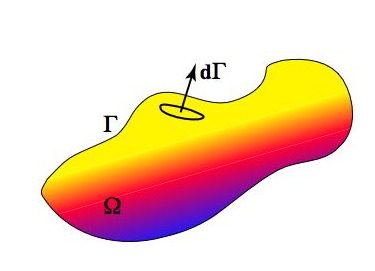
Fig. 3 An arbitrary volume, $\Omega$ of material has a surface $\Gamma$¶

A general conservation law does not distinguish the quantity which is being conserved – it is a mathematical identity. Consider a quantity $\phi$ / unit mass which is carried around by a fluid. We can draw an arbitrary volume, $\Omega$ to contain some amount of this fluid at a given time. We label the surface of the volume $\Omega$ as $\Gamma$, and define an outward vector $\mathbf{d}\boldsymbol{\Gamma}$ which is normal to the surface and represents an infinitesimally small element on the surface. $\dGamma$ has a magnitude equal to the area of this element.

In general, we also need to define a source/sink term, $H$ / unit mass which generates/consumes the quantity $\phi$, and a flux term, $\mathbf{F}$ which is the “leakage” occurs across the surface when the fluid is stationary (e.g. this might represent diffusion of $\phi$). The rate of change of $\phi$ is given by combining the contribution due to the source term, the stationary flux term, and the effect of motion of the fluid.

(1)¶\[ \frac{d}{dt} \int_{\Omega} \rho \phi d\Omega = - \int_{\Gamma} \mathbf{F} \cdot \mathbf{d}\boldsymbol{\Gamma} + \int_{\Omega} \rho H d\Omega - \int _{\Gamma} \rho \phi \mathbf{v} \cdot \mathbf{d}\boldsymbol{\Gamma}\]

where the final term is the change due to the fluid carrying $\phi$ through the volume. Fluxes are positive outward (by our definition of $\mathbf{d}\boldsymbol{\Gamma}$), so a positive flux reduces $\phi$ within $d\Omega$ and negative signs are needed for these terms.

We can use Gauss’ theorem to write surface integrals as volume integrals:

\[\int_{\Gamma} \phi \mathbf{u} \cdot \mathbf{d}\boldsymbol{\Gamma}= \int_{\Omega} \nabla \cdot (\phi \mathbf{u}) d\Omega\]

One more thing: the test surface, $\Gamma$, and volume, $\Omega$ are assumed to be fixed in the lab reference frame which means that the order of integration and differentiation can be interchanged

\[\frac{d}{dt} \int_\Omega \rho \phi d\Omega = \int_\Omega \frac{\partial \rho \phi}{\partial t} d\Omega\]

That means we can write $$ \int_{\Gamma} \mathbf{F} \cdot \mathbf{d}\boldsymbol{\Gamma}+ \int _{\Gamma} \rho \phi \mathbf{v} \cdot \mathbf{d}\boldsymbol{\Gamma}= \int_{\Omega} \nabla \cdot (\mathbf{F} + \rho \phi \mathbf{v}) d\Omega $$

and then rewrite the general conservation equation (1) as

\[ \int_{\Omega} \left[ \frac{d \rho \phi}{dt} + \nabla \cdot (\mathbf{F} + \rho \phi \mathbf{v}) -\rho H \right] d\Omega =0 \]

Now this conservation law has to work no matter what shape we draw for the volume $\Omega$ and so the integral can only be zero for arbitrary $\Omega$ if the enclosed term is zero everywhere, i.e.

(2)¶\[ \frac{d \rho \phi}{dt} + \nabla \cdot (\mathbf{F} + \rho \phi \mathbf{v}) -\rho H =0\]

This is the general conservation rule for any property $\phi$ of a moving fluid. We now consider several quantities and develop specific conservation laws.

Conservation of mass¶

In this case $\phi=1$ because

\[\int_\Omega \rho d\Omega \rightarrow \mbox{mass}\]

Of course, we also know that we cant diffuse or create mass which means $\mathbf{F} = H = 0$ and equation (2) simplifies to give

(3)¶\[ \Red{\frac{\partial \rho}{\partial t} + \nabla \cdot \rho \mathbf{v} = 0}\]

Conservation of (heat) energy¶

The thermal energy / unit mass is $C_p T$ and the conductive heat flux $\mathbf{F}$ is given by $\mathbf{F} = -k \nabla T$, ($k$ is the thermal conductivity).

Then the general conservation equation (2) reduces to this

\[\frac{\partial (\rho C_p T)}{\partial t} + \nabla \cdot \left(-k \nabla T + \rho C_p T \mathbf{v}\right) - \rho H = 0\]

and if we rearrange these terms in the right way we find

\[\frac{C_p T}{\rho} \left[ \frac{\partial \rho}{\partial t} + \nabla \cdot \rho \mathbf{v} \right] + \frac{\partial C_p T}{\partial t} + \mathbf{v} \cdot \nabla C_p T = \frac{1}{\rho} \nabla \cdot k \nabla T + H\]

The term in square brackets is simply the statement of mass conservation and we know immediately that this is zero.

If the heat capacity, $C_p$ and thermal conductivity, $k$ are constants, then the conservation equation becomes

(4)¶\[ \Red{ \left( \frac{\partial T}{\partial t} + \mathbf{v} \cdot \nabla T \right)= \kappa \nabla^2 T + \frac{H}{C_p} }\]

where $\kappa$ is the thermal diffusivity, $\kappa = k/\rho C_p$.

It probably did not go unnoticed that we assumed $\rho$ to be constant to get to this point. It is quite common to assume a material is near-enough incompressible that density changes can be ignored. In fact, this is a reasonable assumption even for air if the velocity is well below the speed of sound. It is also possible to keep assuming incompressibility even when accounting for density variations whose buoyancy effects drive deformation. There is a lot more detail on this in Ricard, 20151 and we will come back to it soon.

A new bit of notation has appeared in the process of this derivation. The the $\mathbf{v} \cdot \nabla$ operator is a derivative that lies along the direction of motion $\mathbf{v}$:

\[\mathbf{v} \cdot \nabla \equiv v_j \frac{\partial}{\partial x_j}\]

For later reference, this is how it looks: $$(\mathbf{v} \cdot \nabla) T = v_1 \frac{\partial T}{\partial x_1} + v_2 \frac{\partial T}{\partial x_2} + v_3 \frac{\partial T}{\partial x_3}$$

The Laplacian, $\nabla^2$, is this expression (for scalar $T$)

\[\nabla^2 T \equiv \frac{\partial^2 T}{\partial x_1^2} + \frac{\partial^2 T}{\partial x_2^2} + \frac{\partial^2 T}{\partial x_3^2}\]

Conservation of momentum¶

Momentum is a vector quantity, so the form of (1) is different. The source term in the momentum equation represents a body force, and the surface flux term represents a stress.

(5)¶\[ \frac{d}{dt}\int_{\Omega} \rho \mathbf{v} d\Omega = - \int_{\Omega} \rho g \hat{\mathbf{z}} d\Omega + \int_{\Gamma} \boldsymbol{\sigma} \cdot \mathbf{d}\boldsymbol{\Gamma}- \int_{\Gamma} \rho \mathbf{v} (\mathbf{v} \cdot \mathbf{d}\boldsymbol{\Gamma}) \]

Gravity provides a body force acting in the vertical direction, $\hat{\mathbf{z}}$. We have introduced the stress tensor, $\boldsymbol{\sigma}$; the force / unit area exerted on an arbitrarily oriented surface with normal $\hat{\mathbf {n}}$ is

\[f_i = \sigma_{ij} n_j\]

The application of Gauss’ theorem, and the equality holds for any choice of the volume gives this result:

(6)¶\[\frac{\partial}{\partial t}(\rho \mathbf{v}) +\rho g \hat{\mathbf{z}} - \nabla \cdot \sigma + \nabla \cdot (\rho \mathbf{v} \mathbf{v}) = 0\]

Vector notation allows us to keep a number of equations written as one single equation. However, at this point, keeping the equations in vector notation makes the situation more confusing. What does that last term on the left hand side of (6) mean ? It is clearer if we use the index notation instead

Equation (6) is equivalent to this:

(7)¶\[\Green{ \frac{\partial \rho v_i}{\partial t}} + \rho g \delta_{i3} - \frac{\partial \sigma_{ij}}{\partial x_j} + \textcolor[rgb]{0.0,0.0,0.7}{ \frac{\partial(\rho v_i v_j)}{\partial x_j}} = 0\]

where that peculiar final term on the left hand side is unambiguous. Repeated indeces in each term are implicitly summed. $\delta_{ij}$ is the kronecker delta which obeys:

\[\begin{split}\delta_{ij} = \begin{cases} 0 & \text{if $i \neq j$}, \\ 1 & \text{if $i = j$}. \end{cases}\end{split}\]

If we expand the derivatives of products of two terms and recombine them in the right way:

\[v_i \left[\Green{ \frac{\partial \rho}{\partial t}} + \Blue{ \frac{\partial \rho v_j}{\partial x_j}} \right] + \Green{ \rho \frac{\partial v_i}{\partial t}} + \Blue{ \rho v_j \frac{\partial v_i}{\partial x_j}} = \frac{\partial \sigma_{ij}}{\partial x_j} -\rho g \delta_{i3}\]

The term in square brackets is, in fact, a restatement of the conservation of mass derived above and must vanish. The remaining terms can now be written out in vector notation as

(8)¶\[\Red{ \rho \left( \frac{\partial \mathbf{v}}{\partial t} + (\mathbf{v} \cdot \nabla) \mathbf{v} \right) = \nabla \cdot \boldsymbol{\sigma} - g\rho\hat{\mathbf{z}} }\]

Note: The $\mathbf{v} \cdot \nabla$ notation we introduced earlier is now an operator on a vector. Written out it looks like this:

\[\begin{split}\begin{split} (\mathbf{v} \cdot \nabla) \mathbf{u} = & \hat{\boldsymbol{\imath}} \left( v_1 \frac{\partial u_1}{\partial x_1} + v_2 \frac{\partial u_1}{\partial x_2} + v_3 \frac{\partial u_1}{\partial x_3} \right) \\ & \hat{\boldsymbol{\jmath}} \left( v_1 \frac{\partial u_2}{\partial x_1} + v_2 \frac{\partial u_2}{\partial x_2} + v_3 \frac{\partial u_2}{\partial x_3} \right) \\ & \hat{\boldsymbol{k}} \left( v_1 \frac{\partial u_3}{\partial x_1} + v_2 \frac{\partial u_3}{\partial x_2} + v_3 \frac{\partial u_3}{\partial x_3} \right) \\ \end{split}\end{split}\]

1: Ricard, Y. “Physics of Mantle Convection.” In Treatise on Geophysics, 23–71. Elsevier, 2015. https://doi.org/10.1016/B978-0-444-53802-4.00127-5.

Geodynamics with Underworld

Conservation Laws¶

Conservation of mass¶

Conservation of (heat) energy¶

Conservation of momentum¶