Non-dimensional equations & dimensionless numbers¶

Before too long it would be a good idea to get a feeling for the flavour of these equations which continual rearrangements will not do — it is necessary to examine some solutions.

First of all it is a good idea to make some simplifications based on the kinds of problems we will want to attack. The first thing to do, as is often the case when developing a model, is to test whether any of the terms in the equations are negligibly small, or dominant. To do this, we are going to need to have some physical insight into the kinds of problems we are going to solve - for example, some terms may be negligible for slow moving flow but not if the flow is fast (but what does ‘fast’ really mean ?)

One trick that is very common in fliud dynamics is to re-scale the equations using units that are in some way natural to the problem we are trying to solve. This helps us to answer the question that came up a moment ago: if a typical velocity is 1, then ‘slow’ is $v \ll 1$ and ‘fast’ is when $v \gg 1$.

Remember that even very rational systems of units like the SI system are still arbitrary and based on the scale of human experience: a metre is not far off the length of a step when we walk, a second is our heartbeat, carry a litre of water when you go walking.

We don’t need to define and name a whole new system of units any time we start analysing a new problem, but the fact that we could do this suggests there is a way to consider the scale of a problem independenly to the underlying character of the way things balance each other as the system changes through time.

What we can do is consider ‘typical values’ for the independent dimensions of a system (mass, length, time, temperature, that sort of thing) which can be used to rescale the standard units. For example, we might rescale all lengths by the size of the system we are studying, $d$ (e.g. mantle thickness or depth of fluid in a lab tank), time according to the characteristic time for diffusion of heat over that distnace, and temperature by maximum temperature difference we observe at the start.

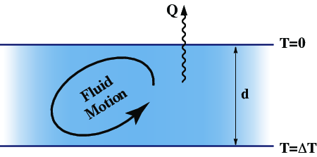
Fig. 4 Consider the fluid motions in a layer of arbitrary depth, $d$. The fluid is assumed to have constant properties such as viscosity, thermal expansivity, thermal diffusivity. Small fluctuations in density due to temperature driven flow. Additional heat is carried (advected) by the flow from the hot boundary to the cool one whenever the fluid is moving.¶

Various scalings result, with the new variables indicated using a prime ($'$).

\[\begin{split} \begin{array}{llll} x = d.x' & \partial / \partial x = (1/d) \partial / \partial x' & \nabla = (1/d) \nabla ' \\ t = (d^2/\kappa) t' & \partial / \partial t = (\kappa/d^2) \partial / \partial t' & \\ T = \Delta T T' & & \\ v = (\kappa / d) v' && \\ p= p_0 + (\eta \kappa / d^2) p' \end{array} \end{split}\]

where $\nabla p_0 = - g \rho_0$

Substituting for all the existing terms in the Navier-Stokes equation ([eq:navstokes]{reference-type=”ref” reference=”eq:navstokes”}) using the equation of state for thermally induced variation in density ([eq:state]{reference-type=”ref” reference=”eq:state”}) gives:

\[ \frac{\rho_0 \kappa}{d^2} \frac{D}{Dt'} \left( \frac{\kappa}{d} \mathbf{v}' \right) = \frac{\eta}{d^2} \acute{\nabla}^2 \left( \frac{\kappa}{d} \mathbf{v}' \right) - \frac{\eta \kappa}{d^3} \acute{\nabla} p' + g \rho_0 \alpha \Delta T T' \hat{\mathbf{z}} \]

Collecting everything together gives

\[ \frac{\rho_0 \kappa^2}{d^3} \frac{D\mathbf{v}'}{Dt'} = \frac{\eta \kappa}{d^3} \acute{\nabla}^2 \mathbf{v}' - \frac{\eta \kappa}{d^3} \acute{\nabla} p' + g \rho_0 \alpha \Delta T T' \hat{\mathbf{z}} \]

Divide throughout by $\eta \kappa / d^3$ gives

\[\begin{split} \begin{aligned} \frac{\rho \kappa}{\eta} \frac{D\mathbf{v}'}{Dt'} & = \acute{\nabla}^2 \mathbf{v}' - \acute{\nabla} p' + \frac{g \rho_0 \alpha \Delta T d^3}{\kappa \eta} T' \hat{\mathbf{z}} \nonumber \\ \textrm{or} \;\;\; \frac{1}{{\rm Pr}} \frac{D\mathbf{v}'}{Dt'} & = \acute{\nabla}^2 \mathbf{v}' - \acute{\nabla} p' + {\rm Ra} T' \hat{\mathbf{z}} \end{aligned} \end{split}\]

$\rm Pr$ is known as the Prandtl number, and $\rm Ra$ is known as the Rayleigh number; both are non-dimensional numbers. By choosing to scale the equations (and this is still perfectly general as we haven’t forced any particular choice of scaling yet), we have condensed the different physical variable quantities into just two numbers. The benefit of this procedure is that it tells us how different quantities trade off against one another. For example, we see that if the density doubles, and the viscosity doubles, then the solution should remain unchanged.

In fact, the main purpose of this particular exercise is about to be revealed. The value of mantle viscosity is believed to lie somewhere between $10^{19}$ and $10^{23}$ ${\rm Pa . s}$, the thermal diffusivity is around $10^{-6}{\rm m}^2{\rm s}^{-1}$, and density around $3300 {\rm kg . m}^{-3}$. This gives a Prandtl number greater than $10^{20}$. Typical estimates for the Rayleigh number are between $10^6$ and $10^8$ depending on the supposed depth of convection, and the uncertain mantle viscosity.

Obviously, the time-dependent term can be neglected for the mantle, since it is at least twenty orders of magnitude smaller than other terms in the equations. The benefit of this is that the nasty advection term for momentum is eliminated – flow in the mantle is at the opposite extreme to turbulent flow. The disadvantage is that the equations now become non-local: changes in the stress field are propogated instantly from point to point which can make the equations a lot harder to solve. This can be counter-intuitive but the consequences are important when considering the dynamic response of the Earth to changes in, for example, plate configurations.

Incidentally, a third, independent dimensionless number can be derived for the thermally driven flow equations. This is the Nusselt number

\[ {\rm Nu} = \frac{Q}{k\Delta T} \]

and is the ratio of actual heat transported by fluid motions in the layer compared to that transported conductively in the absence of fluid motion.

All other dimensionless quantities for this system can be expressed as some combination of the Nusselt, Rayleigh and Prandtl numbers. The Prandtl number is a property of the fluid itself – typical values are: air, $\sim$1; water, $\sim$ 6; non-conducting fluids $10^3$ or more; liquid metal, $\sim$0.1. Rayleigh number and Nusselt number are both properties of the chosen geometry.

Exercise

If the acceleration term is ignored, it means we are assuming the kinetic energy of the flow is small (forces are always in static equilibrium).

Estimate the kinetic energy of the Pacific Plate and compare this value to the average daily energy requirement of an adult human. Also compare this to the heat lost by the Earth in a day.

Does this mean that you could eat an extra-large breakfast and then stop plate tectonics ?

Does the Earth’s rotation matter ?¶

The effect of the Earth’s rotation is very strong in the atmosphere, oceans and in the outer core where Coriolis effects induce rotational flows. In slow-moving, high-viscosity fluids, the effect of rotation is likely to be smaller, but is it negligible like the inertial term ?

To answer that question, we can look at the relative magnitudes of the accelerations in a rotating reference frame, $\{\hat{\mathbf{e}}_i\}$ without having to transform the equations into that reference frame. The vectors are continually transformed by the rotation so that:

\[ \frac{d \hat{\mathbf{e}}_i}{dt} = \boldsymbol{\omega} \times \hat{\mathbf{e}}_i \]

where $\boldsymbol{\omega}$ is the angular velocity of Earth. Then a vector in the rotating reference frame $\mathbf{x} \equiv \left\{ x_i \hat{\mathbf{e}}_i \right\}$ moves at

\[ \left. \frac{d \mathbf{x}}{dt} \right|_0 = \frac{d x_i}{d t} \hat{\mathbf{e}}_i + x_i \frac{d \hat{\mathbf{e}}_i}{dt} \]

in the static reference frame. We can rewrite this as

\[ \left. \frac{d \mathbf{x}}{dt} \right|_0 = \mathbf{v}_R + \boldsymbol{\omega} \times \mathbf{x} \]

where $\mathbf{v}_R$ is the velocity of a point in the rotating reference frame. We can find the acceleration by a further time derivative and we find this:

\[ \boldsymbol\gamma_0 = \boldsymbol\gamma_R + 2 \boldsymbol{\omega} \times \mathbf{v}_R + \boldsymbol{\omega} \times \left( \boldsymbol{\omega} \times \mathbf{x} \right) + \Red{\frac{d \boldsymbol{\omega}}{dt} \times \mathbf{x}} \]

These are the Coriolis, centrifugal and Poincar’e accelerations and the latter we will ignore by assuming changes in rotation are negligible in the case of the modern Earth.

Now we only need to consider the relative magnitude of these terms by estimating characteristic scales. The ratio of the Coriolis term to the imposed gravitational acceleration is, for the Earth,

\[ \frac{2 \omega U} {g} \approx 10^{-13} \]

where $U$ is a typical mantle flow or plate velocity (say 10 cm/yr). Gravitational forces only drive flow when density gradients are present, so a more reliable estimate of the relative magnitude in the case where density variations occur due to temperature would be

\[ \frac{2 \rho \omega U} {\rho \alpha \Delta T g} \approx 10^{-11} \]

This might not be as dramatic a scale separation as for intertia, but it does suggest that the Coriolis term does not play a role in mantle dynamics for the Earth.

The centrifugal acceleration term compared to the gravitational acceleration is

\[ \frac{\omega^2 R_\mathrm{Earth} } {g} \approx 3.10^{-3} \]

which, is clearly not negligible in scale compared to the typical accelerations due to density variations within the Earth. However, this acceleration depends only on the distance from the rotation axis and not on the flow velocity. It is responsible for the equatorial bulge of the Earth which is, to first order, part of the hydrostatic balance that does not influence flow patterns.

There are some more dimensionless numbers at work here. The Rossby number is the ratio of inertial forces to Coriolis forces, and the Eckman number is the ratio of the viscous forces to Coriolis forces.

The stream function¶

For incompressible flows in two dimensions it can be very convenient to work with the stream-function – a scalar quantity which defines the flow everywhere. The stream function is the scalar quantity,$\psi$, which satisfies

\[ v_1 = -\frac{\partial \psi}{\partial x_2} \mathrm{\hspace{1cm}} v_2 = \frac{\partial \psi}{\partial x_1} \label{eq:strmfn} \]

so that, automatically,

\[ \frac{\partial v_1}{\partial x_1} + \frac{\partial v_2}{\partial x_2} = 0 \]

Importantly, computing the following

\[ (\mathbf{v} \cdot \nabla) \psi = v_1 \frac{\partial \psi}{\partial x_1} + v_2 \frac{\partial \psi}{\partial x_2} = \frac{\partial \psi}{\partial x_2} \frac{\partial \psi}{\partial x_1} - \frac{\partial \psi}{\partial x_1} \frac{\partial \psi}{\partial x_2} = 0 \]

tells us that $\psi$ does not change due to advection – in other words, contours of constant $\psi$ are streamlines of the fluid.

Provided we limit ourselves to the xy plane, it is possible to think of equation ([eq:strmfn]{reference-type=”ref” reference=”eq:strmfn”}) as

\[ \mathbf{v} = \nabla \times (\psi \hat{\mathbf{k}}) \]

This form can be used to write down the 2D axisymetric version of equation ([eq:strmfn]{reference-type=”ref” reference=”eq:strmfn”})

\[ \begin{aligned} u_r = -\frac{1}{r}\frac{\partial \psi}{\partial \theta} & & u_\theta = \frac{\partial \psi}{\partial r} \end{aligned} \]

which automatically satisfies the incompressibility condition in plane polar coordinates $$ \frac{1}{r}\frac{\partial}{\partial r}(ru_r) + \frac{1}{r}\frac{\partial u_\theta}{\partial \theta} = 0 $$

Vorticity¶

Vorticity is defined by $$\boldsymbol{\omega} = \nabla \times \mathbf{v}$$

In 2D, the vorticity can be regarded as a scalar as it has only one component which lies out of the plane of the flow.

\[\omega = \frac{\partial v_2}{\partial x_1} - \frac{\partial v_1}{\partial x_2}\]

which is also exactly equal to twice the local measure of the spin in the fluid. Local here means that it applies to an infinitessimal region around the sample point but not to the fluid as a whole.

This concept is most useful in the context of invicid flow where vorticity is conserved within the bulk of the fluid provided the fluid is subject to only conservative forces – that is ones which can be described as the gradient of a single-valued potential.

In the context of viscous flow, the viscous effects acts cause diffusion of vorticity, and in our context, the fact that buoyancy forces result from to (irreversible) heat transport means that vorticity has sources. Taking the curl of the Navier-Stokes equation, and substituting for the vorticity where possible gives

\[\frac{1}{\rm Pr} \left( \frac{D \boldsymbol{\omega}}{D t} - (\boldsymbol{\omega} \cdot \nabla) \mathbf{v} \right) = \eta \nabla ^2 \boldsymbol{\omega} + {\rm Ra} \frac{\partial T}{\partial x_1} \]

The pressure drops out because $\nabla \times \nabla P = 0 \mbox{\hspace{0.5cm}} \forall P$.

Stream-function, vorticity and the biharmonic equation¶

In the context of highly viscous fluids in 2D, the vorticity equation is

\[\nabla ^2 \omega = - Ra \frac{\partial T}{\partial x_1} \label{eq:vorteqn} \]

and, by considering the curl of $(-\partial \psi / \partial x_2, \partial \psi / \partial x_1, 0)$ the stream function can be written

\[\nabla ^2 \psi = \omega \label{eq:psivort} \]

This form is useful from a computational point of view because it is relatively easy to solve the Laplacian, and the code can be reused for each application of the operator. The Laplacian is also used for thermal diffusion – one subroutine for three different bits of physics which is elegant in itself if nothing else.

The biharmonic operator is defined as

\[\nabla^4 \equiv \nabla^2 ( \nabla ^2) \equiv \left( \frac{\partial ^4}{\partial x_1^4} + \frac{\partial ^2}{\partial x_1^2} \frac{\partial ^2}{\partial x_2^2} + \frac{\partial ^4}{\partial x_2^4} \right)\]

The latter form being the representation in Cartesian coordinates.

Using this form, it is easy to show that equations ([eq:vorteqn]{reference-type=”ref” reference=”eq:vorteqn”}) and ([eq:psivort]{reference-type=”ref” reference=”eq:psivort”}) can be combined to give

\[\nabla^4 \psi = -{\rm Ra} \frac{\partial T}{\partial x_1} \label{eq:biharm} \]

Poloidal/Toroidal velocity decomposition¶

The stream-function / vorticity form we have just used is a simplification of the more general case of the poloidal / toroidal velocity decomposition which turns out to be useful when we want to understand the balance of different contributions to the governing equation.

We can make a Helmholtz decomposition of the velocity vector field:

\[\mathbf{u} = \nabla \phi + \nabla \times \mathbf{A}\]

Then for an incompressible flow, since $\nabla \cdot \mathbf{u} = 0$, $$\mathbf{u} = \nabla \times \mathbf{A} \label{eq:curlA}$$

Now suppose there is some direction ($\hat{\mathbf{z}}$) which we expect to be physically favoured in the solutions, we can rewrite [eq:curlA]{reference-type=”ref” reference=”eq:curlA”} as

\[\mathbf{u} = \textcolor[rgb]{0.7,0.0,0.0}{\nabla \times(\Psi \hat{\mathbf{z}})} + \textcolor[rgb]{0.0,0.0,0.7}{ \nabla \times\nabla \times(\Phi \hat{\mathbf{z}})} \label{eq:poltor}\]

Where the first term on the right is the [Toroidal]{style=”color: 0.7,0.0,0.0”} part of the flow, and the second term is the [ Poloidal]{style=”color: 0.0,0.0,0.7”} part. Why is this useful ? Let’s substitute ([eq:poltor]{reference-type=”ref” reference=”eq:poltor”}) into the Stokes’ equation for a constant viscosity fluid

\[\eta \nabla^2 \mathbf{u} - \nabla p = g \rho \hat{\mathbf{z}} \label{eq:cvstokes}\]

where $\hat{\mathbf{z}}$ is the vertical unit vector (defined by the direction of gravity) and is clearly the one identifiable special direction, then equate coefficients in the $\hat{\mathbf{z}}$ direction, and using the following results:

\[\hat{\mathbf{z}} \cdot \nabla \times \nabla^2 \mathbf{u} = - \nabla^2 \nabla_h^2\Psi\]

\[\hat{\mathbf{z}} \cdot \nabla \times \nabla \times \nabla^2 \mathbf{u} = \nabla^2 \nabla^2 \nabla_h^2\Phi\]

where

\[\nabla_h = \left( \frac{\partial}{\partial x}, \frac{\partial}{\partial y}, 0 \right)\]

is a gradient operator limited to the plane perpendicular to the special direction, $\hat{\mathbf{z}}$.

If we first take the curl of ([eq:cvstokes]{reference-type=”ref” reference=”eq:cvstokes”}), and look at the $\hat{\mathbf{z}}$ direction,

\[\hat{\mathbf{z}} \cdot \eta \nabla \times \nabla^2 \mathbf{u} = -\eta \nabla^2 \nabla_h^2\Psi = \hat{\mathbf{z}} \cdot \left( g \nabla \times \left( \rho \hat{\mathbf{z}}\right)\right) = 0 \]

we see that there is no contribution of the toroidal velocity field to the force balance. This balance occurs entirely through the poloidal part of the velocity field. If we take the curl twice and, once again, look at the $\hat{\mathbf{z}}$ direction:

\[\hat{\mathbf{z}} \cdot \eta \nabla \times \nabla \times \nabla^2 \mathbf{u} = \eta \nabla^2 \nabla^2 \nabla_h^2 \Phi = \hat{\mathbf{z}} \cdot g \nabla \times \nabla \times \left( \rho \hat{\mathbf{z}}\right) = \nabla_h^2 (\rho g)\]

Which is the 3D equivalent of the biharmonic equation that we derived above.

Note: if the viscosity varies in the $\hat{\mathbf{z}}$ direction, then this same decoupling still applies: bouyancy forces do not drive any toroidal flow. Lateral variations in viscosity (perpendicular to $\hat{\mathbf{z}}$) couple the buoyancy to toroidal motion. This result is general in that it applies to the spherical geometry equally well assuming the radial direction (of gravity) to be special.

Sample solutions¶

A number of related solutions exist to problems such as unstable layering breaking down, buckling of viscous layers and rebound of topography when surface loading changes.

Rayleigh-Taylor Instability & Diapirism¶

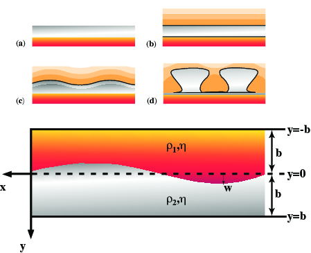
Fig. 5 Salt diapirs result when a buried layer of salt(a,b) becomes convectively unstable and rises through the overlying sediment layers (c,d). The idealized geometry for the Rayleigh-Taylor instability problem is outlined in the lower diagram¶

Diapirism is the buoyant upwelling of rock which is lighter than its surroundings. This can include mantle plumes and other purely thermal phenomena but it often applied to compositionally distinct rock masses such as melts infiltrating the crust (in the Archean) or salt rising through denser sediments.

Salt layers may result from the evaporation of seawater. If subsequent sedimentation covers the salt, a gravitionally unstable configuration results with heavier material (sediments) on top of light material (salt). The rheology of salt is distinctly non-linear and also sensitive to temperature. Once buried, the increased temperature of the salt layer causes its viscosity to decrease to the point where instabilities can grow. Note, since there is always a strong density contrast between the two rock types, the critical Rayleigh number argument does not apply – this situation is always unstable, but instabilities can only grow at a reasonable rate once the salt has become weak.

The geometry is outlined above in Figure ( 2{reference-type=”ref” reference=”fig:raytay”}). We suppose initially that the surface is slightly perturbed with a form of

\[w_m = w_{m0} \cos kx\]

where $k$ is the wavenumber, $k=2\pi / \lambda$, $\lambda$ being the wavelength of the disturbance. We assume that the magnitude of the disturbance is always much smaller than the wavelength.

The problem is easiest to solve if we deal with the biharmonic equation for the stream function. Experience leads us to try to separate variables and look for solutions of the form

\[\psi = \left( A \sin kx + B \cos kx \right ) Y(y)\]

where the function $Y$ is to be determined. The form we have chosen for $w_m$ in fact means $A=1,B=0$ which we can assume from now on to simplify the algebra.

Substituting the trial solution for $\psi$ into the biharmonic equation gives

\[\frac{d^4 Y}{d y^4} -2k^2 \frac{d^2 Y}{dy^2} +k^4 Y = 0\]

which has solutions of the form

\[Y = A \exp(m y)\]

where $A$ is an arbitrary constant. Subtituting gives us an equation for $m$

\[m^4 - 2 k^2 m^2 + k^4 = (m^2 - k^2)^2 = 0 \label{eq:diapaux}$$ or $$m = \pm k\]

Because we have degenerate eigenvalues (i.e. of the four possible solutions to the auxilliary equation ([eq:diapaux]{reference-type=”ref” reference=”eq:diapaux”}), two pairs are equal) we need to extend the form of the solution to

\[Y = (By+A) \exp(m y)\]

to give the general form of the solution in this situation to be

\[\begin{split}\begin{aligned} \psi &= \sin kx \left( A e^{-ky} + B y e^{-ky} + C e^{ky} + D y e^{ky} \right) \label{eq:biharmsoln1} \\ \mathrm{or, equivalently} \psi &= \sin kx \left( A_1 \cosh ky + B_1 \sinh ky + C_1 y \cosh ky + D_1 y \sinh ky \right) \label{eq:biharmsoln2} \end{aligned}\end{split}\]

This equation applies in each of the layers separately. We therefore need to find two sets of constants $\{A_1,B_1,C_1,D_1\}$ and $\{A_2,B_2,C_3,D_4\}$ by the application of suitable boundary conditions. These are known in terms of the velocities in each layer, $\mathbf{v}_1 = \mathbf{i} u_1 +\mathbf{j} v_1$ and $\mathbf{v}_2 = \mathbf{i} u_2 +\mathbf{j} v_2$:

\[\begin{split}\begin{aligned} u_1 = v_1 &= 0 \mathrm{\hspace{1cm} on \hspace{1cm}} y = -b \\ u_2 = v_2 &= 0 \mathrm{\hspace{1cm} on \hspace{1cm}} y = b \end{aligned}\end{split}\]

together with a continuity condition across the interface (which we assume is imperceptibly deformed

\[u_1 = u_2 \mathrm{\hspace{1cm} and \hspace{1cm}} v_1 = v_2 \mathrm{\hspace{1cm} on \hspace{1cm}} y = 0\]

The shear stress ($\sigma_{xy}$) should also be continuous across the interface, which, if we assume equal viscosities, gives

\[\frac{\partial u_1}{\partial y} + \frac{\partial v_1}{\partial x} = \frac{\partial u_2}{\partial y} + \frac{\partial v_2}{\partial x} \mathrm{\hspace{1cm} on \hspace{1cm}} y = 0 \]

and, to simplify matters, if the velocity is continuous across $y=0$ then any velocity derivatives in the $x$ direction evaluated at $y=0$ will also be continuous (i.e. $\partial v_2 / \partial x = \partial v_1 / \partial x$).

The expressions for velocity in terms of the solution ([eq:biharmsoln2]{reference-type=”ref” reference=”eq:biharmsoln2”}) are

\[\begin{split}\begin{aligned} u = -\frac{\partial \psi}{\partial y} & = -\sin kx \left( (A_1 k + D_1 + C_1 k y) \sinh ky + (B_1 k + C_1 + D_1 ky) \cosh ky \right) \\ v = \frac{\partial \psi}{\partial x} & = k \cos kx \left( (A_1 +C_1 y)\cosh ky + (B_1 +D_1 y) \sinh ky \right) \end{aligned}\end{split}\]

From here to the solution requires much tedious rearrangement, and the usual argument based on the arbitrary choice of wavenumber $k$ but we finally arrive at

\[\begin{split}\begin{gathered} \psi_1 = A_1 \sin kx \cosh ky + \\ A_1 \sin kx \left[ \frac{y}{k b^2} \tanh kb \sinh ky + \left( \frac{y}{b} \cosh ky \frac{1}{kb} \sinh ky \right) \cdot \left( \frac{1}{kb} + \frac{1}{\sinh bk \cosh bk} \right) \right] \times \\ \left[ \frac{1}{\sinh bk \cosh bk} - \frac{1}{(b^2k^2} \tanh bk \right] ^{-1} \label{eq:raytays1} \end{gathered}\end{split}\]

The stream function for the lower layer is found by replacing $y$ with $-y$ in this equation. This is already a relatively nasty expression, but we haven’t finished since the constant $A_1$ remains. This occurs because we have so far considered the form of flows which satisfy all the boundary conditions but have not yet considered what drives the flow in each layer.

To eliminate $A_1$, we have to consider the physical scales inherent in the problem itself. We are interested (primarily) in the behaviour of the interface which moves with a velocity $\partial w / \partial t$. As we are working with small deflections of the interface,

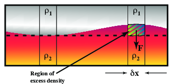
\[\frac{\partial w}{\partial t} = \left. v \right|_{y=0}\]

Fig. 6 The restoring force for a stable layering is proportional to the excess density when a fluid element is displaced across the boundary¶

Consider what happens when the fluid above the interface is lighter than the fluid below – this situation is stable so we expect the layering to be preserved, and if the interface is disturbed the disturbance to decay. This implies that there must be a restoring force acting on an element of fluid which is somehow displaced across the boundary at $y=0$ (Figure 3{reference-type=”ref” reference=”fig:raytay2”}).

This restoring force is due to the density difference between the displaced material and the layer in which it finds itself. The expression for the force is exactly that from Archimedes principle which explains how a boat can float (only in the opposite direction)

\[\left. F_2 \right|_{y=0} = \delta x g w (\rho_2 - \rho_1)\]

which can be expressed as a normal stress difference (assumed to apply, once again, at the boundary). The viscous component of the normal stress turns out to be zero – proven by evaluating $\partial v / \partial y$ at $y=0$ using the expression for $\phi$ in equation ([eq:raytays1]{reference-type=”ref” reference=”eq:raytays1”}). Thus the restoring stress is purely pressure

\[\left. P_2 \right|_{y=0} = g w (\rho_2 - \rho_1)\]

The pressure in terms of the solution (so far) for $\psi$ is found from the equation of motion in the horizontal direction (substituting the stream function formulation) and is then equated to the restoring pressure above.

\[(\rho_1-\rho_2) g w = -\frac{4 \eta k A_1}{b} \cos kx \left(\frac{1}{kb} + \frac{1}{\sinh bk \cosh bk} \right) \cdot \left( \frac{1}{\sinh bk \cosh bk} - \frac{1}{(b^2k^2} \tanh bk \right)^{-1} \]

which allows us to substitute for $A_1$ in our expression for $\partial w / \partial t$ above. Since $A_1$ is independent of $t$, we can see that the solution for $w$ will be of a growing or decaying exponential form with growth/decay constant coming from the argument above.

\[w(t) = w_0 \exp((t-t_0)/\tau)\]

where

\[\tau = \frac{4 \eta}{(\rho_1-\rho_2) g b} \left( \frac{1}{kb} + \frac{1}{\sinh bk \cosh bk} \right) \cdot \left( \frac{1}{k^2b^2} \tanh kb - \frac{1}{\sinh kb \cosh kb} \right)^{-1} \]

So, finally, an answer – the rate at which instabilities on the interface between two layers will grow (or shrink) which depends on viscosity, layer depth and density differences, together with the geometrical consideration of the layer thicknesses.

A stable layering results from light fluid resting on heavy fluid; a heavy fluid resting on a light fluid is always unstable (no critical Rayleigh number applies) although the growth rate can be so small that no deformation occurs in practice. The growth rate is also dependent on wavenumber. There is a minimum in the growth time as a function of dimensional wavenumber which occurs at $k b = 2.4$, so instabilities close to this wavenumber are expected to grow first and dominate.

Remember that this derivation is simplified for fluids of equal viscosity, and layers of identical depth. Remember also that the solution is for infinitessimal deformations of the interface. If the deformation grows then the approximations of small deformation no longer hold. This gives a clue as to how difficulties dealing with the advection term of the transport equations arise.

At some point it becomes impossible to obtain meaningful results without computer simulation. However, plenty of further work has already been done on this area for non-linear fluids, temperature dependent viscosity &c and the solutions are predictably long and tedious to read, much less solve. When the viscosity is not constant, the use of a stream function notation is not particularly helpful as the biharmonic form no longer appears.

The methodology used here is instructive, as it can be used in a number of different applications to related areas. The equations are similar, the boundary conditions different.

Post-Glacial Rebound¶

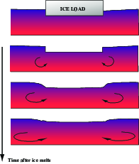
Fig. 7 The relaxation of the Earth’s surface after removal of an ice load.¶

In the postglacial rebound problem, consider a viscous half space with an imposed topography at $t=0$. The ice load is removed at $t=0$ and the interface relaxes back to its original flat state.

This can be studied one wavenumber at a time — computing a decay rate for each component of the topography. The intial loading is computed from the fourier transform of the ice bottom topography.

The system is similar to that of the diapirs except that the loading is now applied to one surface rather than the interface between two fluids.

Phase Changes in the mantle¶

A different interface problem is that of mantle phase changes. Here a bouyancy anomaly results if the phase change boundary is distorted. This can result from advection normal to the boundary bringing cooler or warmer material across the boundary.

The buoyancy balance argument used above can be recycled here to determine a scaling for the ability of plumes/downwellings to cross the phase boundary.

Kernels for Surface Observables¶

The solution method used for the Rayleigh Taylor problem can also be used in determining spectral Green’s functions for mantle flow in response to thermal perturbations. This is a particularly abstract application of the identical theory.

Folding of Layered (Viscous) Medium¶

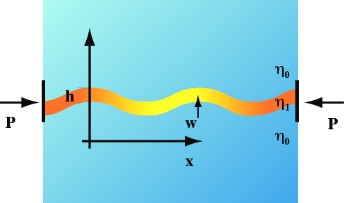
Fig. 8 Instability in a thin, viscous layer compressed from both ends.¶

If a thin viscous layer is compressed from one end then it may develop buckling instabilities in which velocities grow perpendicular to the plane of the layer.

If the layer is embedded between two semi-infinite layers of viscous fluid with viscosity much smaller than the viscosity of the layer, then Biot theory tells us the wavelength of the initial buckling instability, and the rate at which it grows.

The fold geometry evolves as

\[w=w_m \cos(kx) e^{\frac{t}{\tau_a}}\]

where

\[\tau_a = \frac{1}{\bar{P}}\left[ \frac{4 \eta_0}{k} + \frac{\eta_1 h^3}{3k^2} \right]\]

and the fastest growing wavenumber is

\[k = \frac{6}{h}\left( \frac{\eta_1}{\eta_0} \right)^{\frac{1}{3}}\]

For large deformations we eventually must resort to numerical simulation.

Gravity Currents¶

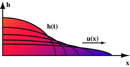
Fig. 9 A gravity current is the spreading of a dense fluid under its own weight across a horizontal surface (or a buoyant fluid under a surface). Open the fridge door and the cold air falls out as a gravity current.¶

Gravity currents can occur when a viscous fluid flows under its own weight as shown in Figure 6{reference-type=”ref” reference=”fig:gcurr1”}.

We assume that the fluid has constant viscosity, $\eta$ and that the length of the current is considerably greater than its height. The fluid is embedded in a low viscosity medium of density $\rho-\Delta \rho$ where $\rho$ is the density of the fluid itself.

The force balance is between buoyancy and viscosity. The assumptions of geometry allow us to simplify the Stokes equation by assuming horizontal pressure gradients due to the surface slope drive the flow.

\[\nabla p = \eta\nabla^2 u \approx g \Delta \rho \frac{\partial h}{\partial x}\]

We assume near-zero shear stress at the top of the current to give

\[\frac{\partial u}{\partial z} (x,h,t) = 0\]

and zero velocity at the base of the current. Hence

\[u(x,z,t) = -\frac{1}{2} \frac{g \Delta \rho}{\eta} \frac{\partial h}{\partial x} z(2h-z)\]

Continuity integrated over depth implies

\[\frac{\partial h}{\partial t} + \frac{\partial }{\partial x} \int_0^h u dz = 0\]

Combining these equations gives

\[\frac{\partial h}{\partial t} -\frac{1}{3} \frac{g \Delta \rho}{\eta} \frac{\partial }{\partial x} \left( h^3 \frac{\partial h}{\partial x} \right) = 0\]

Finally, a global constraint fixes the total amount of fluid at any given time

\[\int_0^{x_N(t)} h(x,t)dx = qt^\alpha\]

The latter term being a fluid source at the origin, and $x_{N(t)}$ the location of the front of the current. A similarity variable is the key to solving this problem:

\[\nu = \left( \frac{1}{3} g\Delta \rho q^3 / \eta \right)^{-\frac{1}{5}} x t^{-(3\alpha +1) / 5}\]

giving a solution of the form

\[h(x,t) = \nu_N^{2/3} (3q^2 \eta / (g\Delta\rho))^{1/5} t^{(2\alpha -1) / 5} \phi(\nu/\nu_N)\]

where $\nu_N$ is the value of $\nu$ at $x=x_N(t)$. Substituting into the equation for $\partial h / \partial t$ we find that $\phi(\nu/\nu_N)$ satisfies

\[\phi({\nu}/{\nu_N}) = \left[ \frac{3}{5}(3\alpha+1)\right]^{\frac{1}{3}} \left(1-\frac{\nu}{\nu_N} \right)^{\frac{1}{3}} \left[ 1 - \frac{3\alpha-4}{24(3\alpha+1)}\left(1-\frac{\nu}{\nu_N} \right) + O \left(1-\frac{\nu}{\nu_N} \right)^2 \right]\]

Which has an analytic solution if $\alpha=0$ (only constant sources or sinks)

\[\begin{split}\begin{split} \phi({\nu}/{\nu_N}) &= \left( \frac{3}{10}\right)^{\frac{1}{3}} \left( 1-\left(\frac{\nu}{\nu_N}\right)^2 \right)^{\frac{1}{3}} \\ \nu_N &= \left[ \frac{1}{5} \left( \frac{3}{10}\right)^{\frac{1}{3}} \pi^{\frac{1}{2}} \Gamma (1/3) / \Gamma (5/6) \right]^{-\frac{3}{5}} = 1.411 \end{split} \end{split}\]

For all other values of $\alpha$ numerical integration schemes must be used for $\phi$.

It is also possible to obtain solutions if axisymmetric geometry is used.

Geodynamics with Underworld

Non-dimensional equations & dimensionless numbers¶

Does the Earth’s rotation matter ?¶

The stream function¶

Vorticity¶

Stream-function, vorticity and the biharmonic equation¶

Poloidal/Toroidal velocity decomposition¶

Sample solutions¶

Rayleigh-Taylor Instability & Diapirism¶

Post-Glacial Rebound¶

Phase Changes in the mantle¶

Kernels for Surface Observables¶

Folding of Layered (Viscous) Medium¶

Gravity Currents¶